Sales & Demand Forecasting for Inventory Planning

A time-series forecasting model on nine years of monthly sales data, built to drive inventory and staffing decisions rather than just predict a number.

7.97%Holdout forecast error (MAPE)

106%Peak-to-trough seasonal swing

+78.9%Underlying growth, first yr to last

~234,600Units forecast, next 12 months

Overview

Built a demand-forecasting pipeline on nine years of monthly sales history to show how a forecasting model becomes concrete inventory and staffing guidance rather than a standalone number. The same methodology — decompose seasonality, validate on a holdout, then forecast forward — applies directly to any retailer, dealer network, or distributor's monthly sales series.

Method

Python-based time-series pipeline using Holt-Winters exponential smoothing (additive trend, multiplicative seasonality)
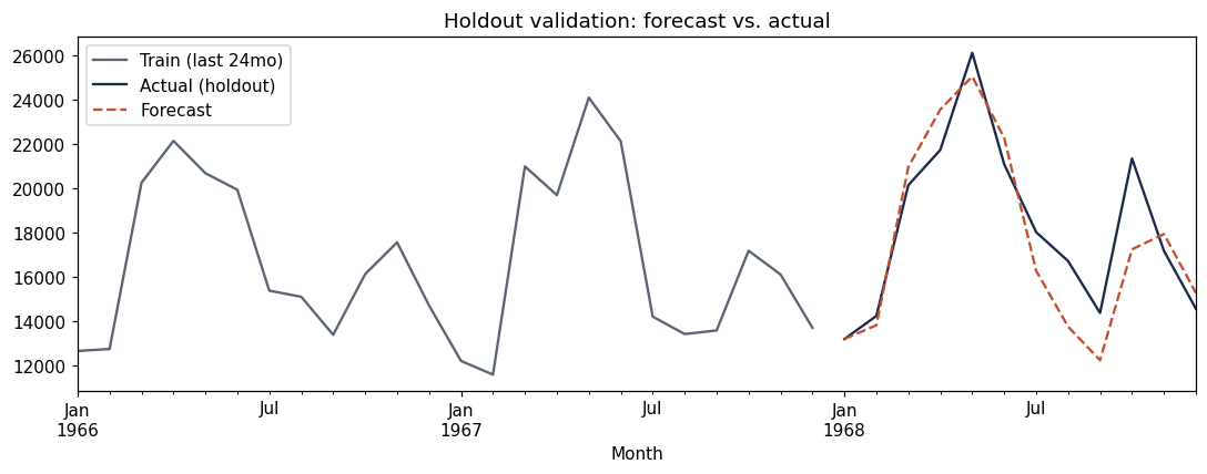
Held out the final 12 months to validate forecast accuracy before generating a forward-looking forecast
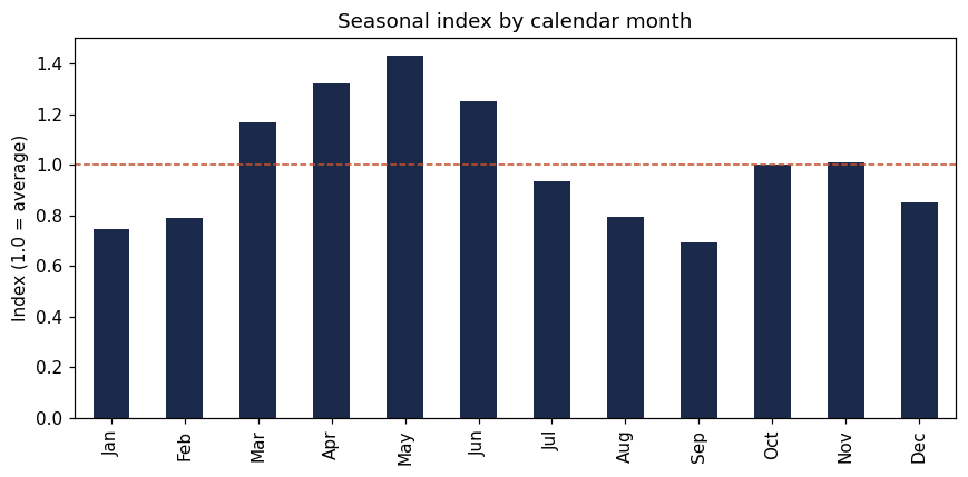
Decomposed the series to separate month-by-month seasonality from the underlying growth trend

Results

Line chart comparing the model's 12-month holdout forecast against actual sales — 12-month holdout validation: the forecast (dashed) tracks the actual sales trajectory closely enough to plan against.

Bar chart of the seasonal index by calendar month — Seasonal index by calendar month — May peaks at 1.4x average, September troughs at 0.7x.

Line chart of the 12-month forward sales forecast — 12-month forward forecast, built on the full nine-year history.

Forecast vs. trailing actuals
Period	Total units
Last actual 12 months	218,738
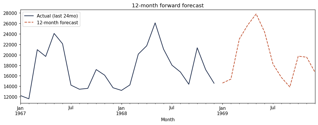
Forecast, next 12 months	234,605 (+7.2%)

Key Findings

Forecast validated against a 12-month holdout at 7.97% MAPE — accurate enough to plan inventory and staffing against, with a known error margin
Strong, consistent seasonality: sales peak in May (+43% vs. average) and trough in September (−30%), a swing of roughly 106% between the two — a pattern that should directly shape stocking and staffing schedules
Underlying demand grew 78.9% comparing the first and last 12-month periods of the series, separate from the seasonal swings
12-month forward forecast: ~234,600 units, a ~7.2% increase over the prior 12 months

Deliverable

Full analysis delivered as a Jupyter notebook with the forecast, seasonal decomposition, and holdout validation, including charts.